2023-10-28

【TOEIC】相関接続詞の例文まとめ

英語

こんてんつ

TOEICに頻出の相関接続詞の例文を幾つか紹介する。

both A and B
either A or B
neither A nor B
not only A but also B

例文

both A and B

Both Taro and John like apple. （TaroもJohnもリンゴが好きだ。）
I think both you and I are mistaken. （あなたと私の両方が間違っていると思います。）
Taro can both speak and write Japanese.

either A or B

Either Taro or John likes apple. （TaroかJohnのどちらかはリンゴが好きだ。）
I think she is either a president or a director.

neither A nor B

Neither this book nor that one was very good. （この本もあの本もあまりよくなかった。）
Neither Taro nor John has enough money to pay the rent.
Neither Taro nor his brothers have enough money to pay the rent.
The doctor advised me neither to drink nor to smoke.
The boy neither admits nor denies that he told a lie. （その少年は嘘をついたことを認めてもいないし、否定もしていない。）

not only A but also B

I think not only you but also I am mistaken. （あなただけでなく私も間違っていると思います。）
He speaks not only English but also Spanish.
Not only English but also Spanish does he speak. （倒置）
I was fascinated not only by her smile but also by her voice.

2023-09-24

平行軸の定理を使ってT字梁の断面二次モーメントを求める

材料力学

こんてんつ

※本記事では厳密な一般解の証明までは出来ませんでした。数値的に定理から求められることを検証します。

T字はりの断面2次モーメント $I$ の公式は、

$\displaystyle \begin{eqnarray} && I = \frac{1}{3}\{te_1^3 + be_2^3 - (b-t)(e_2-s)^3\} \\ && e_1= d - \frac{d^2 t + s^2(b-t)}{2(bs+ht)} \\ && e_2= \frac{d^2 t + s^2(b-t)}{2(bs+ht)}\\ \end{eqnarray}$

などとして、与えられることをよく目にする。この式から出てくる値が、平行軸の定理からを利用して求められることについて解説する。

平行軸の定理

断面二次モーメントに関する平行軸の定理

梁曲げのたわみの計算式などでは、最小値となる図芯を通る断面二次モーメント $I_z$ を用いる必要がある。これは、任意の $z^{'}$ 軸周りの断面二次モーメント $I_{z^{'}}$ を求めた後、図芯までの距離の二乗 ${\bar{y}}^2$ に、断面積 $A$ を乗じたものを引くことで求められる。平行軸の定理は次式である。

$\displaystyle I_z = I_{z^{'}} - ({\bar{y}})^2 A$

（参考）高校力学における平行軸の定理

平行軸の定理は、高校物理学のモーメントの章にて登場している。質量 $M$ の剛体の任意の軸のまわりの慣性モーメント $I$ は、その軸と重心の距離を $h$ 、質量中心を通りその軸に平行な軸のまわりの慣性モーメントを $I_G$ とするとき、

$\displaystyle I = I_G + M h^2$

で与えられる。

平行軸の定理を利用したT字梁の断面二次モーメントの導出

次のようなT字梁を設定する。図芯を通る断面二次モーメント $I_z$ は、任意の $z^{'}$ 軸周りの断面二次モーメント $I_{z^{'}}$ から、平行軸の定理により図芯までの距離の二乗 ${\bar{y}}^2$ に、断面積 $A$ を乗じたものを引くことで、

$\displaystyle I_z = I_{z^{'}} - ({\bar{y}})^2 A$

で与えられる。ここで、 $I_{z^{'}}$ は断面二次モーメントの定義によって、

$\displaystyle \begin{eqnarray} I_z &=& \int y^2 dA - ({\bar{y}})^2 A \\ &=& \left( \int_0^s y^2 \cdot b dy + \int_s^d y^2 \cdot t dy \right)- ({\bar{y}})^2 A \end{eqnarray}$

となる。ここで、図芯までの距離 $\bar{y}$ は、断面一次モーメントとも呼ばれ、

$\displaystyle \bar{y} = \frac{\int y dA}{A} = \frac{ \int_0^s y \cdot b dy + \int_s^d y \cdot t dy } {A}$

という形で表すことが出来る。以上より、

$\displaystyle \begin{eqnarray} I_z &=& \left( \int_0^s y^2 \cdot b dy + \int_s^d y^2 \cdot t dy \right)- \left( \frac{ \int_0^s y \cdot b dy + \int_s^d y \cdot t dy } {A} \right) ^2 A \end{eqnarray}$

という形で図芯を通る断面二次モーメント $I_z$ を求めることが出来る。ここで、仮に

$\displaystyle \begin{eqnarray} b &=& 100\\ d &=& 20\\ s &=& 10\\ t &=& 10 \end{eqnarray}$

とすると、

$\displaystyle \begin{eqnarray} I_z &=& \left( 33333.3 + 23333.3 \right)- \left( \frac{ 5000 + 1500 } {1100} \right) ^2 1100 \\ &=& 18257.5 \end{eqnarray}$

となる。冒頭示した式との計算値とも一致し、平行軸の定理を使ってT字梁の断面二次モーメントを導出する式を示すことが出来た。

2023-06-03

【スプレッドシート】縦一列に長いデータを複数列に変換する

スプレッドシート

こんてんつ

縦一列に並んだデータがあるとする。このデータを、指定行で折り返させ、複数列に変換するための方法を示す。

例題

次の図の様に、A列に長いデータが存在するとする。このデータを、4行おきにB列、C列、…のように横に移動させることを考える。

方法

B1列に次の様な関数を記入し、オートフィルで周りに広げればよい。4*(ROW()-1)+(COLUMN()-1)の4の部分を折り返したい行数に一致させることがポイント。 =INDEX($A:$A,4*(ROW()-1)+(COLUMN()-1),0)

解説

INDEXは、INDEX(参照, 行, 列)として、値を取得してこれる。4*(ROW()-1)+(COLUMN()-1)におけるn=4の部分で、記入している行のn倍の行を取得して、(COLUMN()-1)分足した行の値を取得してくる。

利用の用途

例えば、次の様な、氏名・年齢・住所の様に縦に並んだデータを、横に並べるときなどに有用である。

2023-05-21

【Python】copyとdeepcopyの違い

python

こんてんつ

copyモジュールの浅いcopyと深いコピーdeepcopyの違いについて例を使って説明する。

結論

deepcopy：新しい複合オブジェクトを作成し、その中にコピーを挿入する。よって、元のオブジェクトとコピーされたオブジェクトは完全に独立している。
copy：新しい複合オブジェクトを作成し、その中に元のオブジェクトに対する参照を挿入する。よって、コピーされたオブジェクトは元のオブジェクトの参照のみである。

例

コード

import copy

original_list = [[1, 2], [3, 4]]
normal_copy = copy.copy(original_list)
deep_copy = copy.deepcopy(original_list)

original_list[0][0] = 99

print(f'Original list: {original_list}')
print(f'normal_copy: {normal_copy}')
print(f'Deep copy: {deep_copy}')

実行結果

解説

original_listというリストを用意し、copyとdeepcopyによって浅いコピーと深いコピーを作成した。その後、original_listの最初の要素を99に変更した。この変更は、copyにも影響するが、deep_copyには影響しない。

よって、浅いコピーは元のオブジェクトの中にあるオブジェクトを参照するため、元のオブジェクトが変更されると、浅いコピーも変更さる。一方、深いコピーは元のオブジェクトと完全に独立しているため、元のオブジェクトが変更されても、深いコピーは変更されない。

2023-05-18

バッチファイルで親フォルダ内の子フォルダのファイルを一括でリネームする

コマンドプロンプト/バッチ

こんてんつ

親フォルダ内の子フォルダに存在するファイルを、「親フォルダ名+連番」でリネームするバッチファイルのコードを示す。以下の.batファイルを親フォルダ内に置いて実行することで、ファイル名を変更することが出来る。

コード

例題

下記のフォルダの中に、テスト用のファイルとバッチファイルを用意する。

↓

これを、下記の様に「親フォルダ名+連番」でリネームする。

↓

サマリー

@echo off
setlocal enabledelayedexpansion

:: 現在のディレクトリを表示
echo ##### ##### ##### WARNING !!!!! ##### ##### #####
echo ##### ##### ##### WARNING !!!!! ##### ##### #####
echo ##### ##### ##### WARNING !!!!! ##### ##### #####
echo.
echo Current Directory is 
echo %CD%
echo.

:: 確認メッセージを表示
echo Can I execute? [y/n]
set /p "confirm="

echo.

if /i "%confirm%"=="y" (
    :: 初期化
    set "lastParent="
    set "count=0"

    :: 全てのファイルに対して繰り返し処理を行う
    for /r %%i in (*) do (
        if not "%%~nxi"=="%~nx0" ( :: .batファイル自身のリネームを回避
        echo I will rename %%~nxi :: 確認用
            :: 親フォルダ名を取得
            set "parent=%%~dpi"
            set "parent=!parent:~0,-1!"   :: 末尾の\を除去
            for %%j in ("!parent!") do set "parent=%%~nj"   :: フォルダ名だけにする

            :: 親フォルダが変わった場合はカウントをリセットする
            if not "!parent!"=="!lastParent!" set "count=1"

            :: リネームする際の接頭辞と接尾辞を設定
            set "prefix=!parent!_"
            set "suffix=%%~xi"

            :: 0埋めして連番を設定
            set "number=!count!"
            if !count! LSS 100 set "number=0!count!"
            if !count! LSS 10 set "number=00!count!"

            :: 新しいファイル名を作成
            set "newName=!prefix!!number!!suffix!"

            :: ファイルをリネーム
            ren "%%i" "!newName!"

            :: カウントを更新
            set /a "count+=1"
            set "lastParent=!parent!"
        )
    )
    echo Finished.
) else (
    echo Canceled.
)

pause

解説

変数の設定

set "lastParent="：前回処理したファイルの親フォルダ名を記憶する変数。

for文によるすべてのファイルへの処理

for /r %%i in (*) do (：for /r の/rは「サブディレクトリを再帰的に処理する」という意味のオプション。指定されたディレクトリ以下のすべてのサブディレクトリについて、forコマンドで処理を繰り返す。

親フォルダ名の取得

set "parent=%%~dpi"：parent変数に現在のファイルの親フォルダまでのフルパスを取得。%%~dpiは、%%i変数のドライブ名とディレクトリ名を表し、~dpはドライブ名とディレクトリ名を抽出するための修飾子。
for %%j in ("!parent!") do set "parent=%%~nj"：このままではparent変数がフルパスなので、親フォルダ名だけにするコマンド。set "parent=%%~nj"は、%%j変数に格納されたフルパスから、親フォルダ名のみを抽出してparent変数に設定できる。

リネームの設定

set "prefix=!parent!_"：「親フォルダ名+_（アンダーバー）」として定義しておく。
set "suffix=%%~xi"：suffixを%%iの拡張子として定義する。%%~xiは%%iの拡張子を表す。
set "newName=!prefix!!number!!suffix!"とren "%%i" "!newName!"：これによって、ファイル%%iをnewNameにリネームする。

未解決問題

echo I will rename %%~nxi :: 確認用を省略した場合、何故か「指定されたドライブが見つかりません。」というメッセージが出てくる（動作には問題が無い）。原因が分かる方がいらっしゃいましたら、ご教示いただけますと幸いです。

2023-04-25

スプレッドシートで複数のシートを結合する（VLOOKUP）

スプレッドシート

こんてんつ

スプレッドシートでVLOOKUP関数を使って複数のシートを結合する簡単な例を紹介する。これで、SQLチックに複数のシートをくっつけられる。

例題

次の2つのシートがあったとする。「シート1」のC列目に、IDに対応するシート2のAgeを結合することを考える。

解答

=VLOOKUP(A2,シート2!A:B, 2, FALSE)と入力することで、シート2!A:B範囲のA2セルの値と一致する値を検索し、2列目に存在するAgeを返すことが出来る。これをオートフィルする。

尚、FALSEは近似値の検索をしないことを意味する。

2022-12-25

【R】ggplotで散布図を書く時のチートシート

こんてんつ

ggplotで散布図を書く時の備忘録である。

基本編
条件合致のみプロット編
軸の調整編
軸ラベルやタイトル編
点の見た目の変更編
色の調整編
並べてプロット編
回帰直線編

チートシート

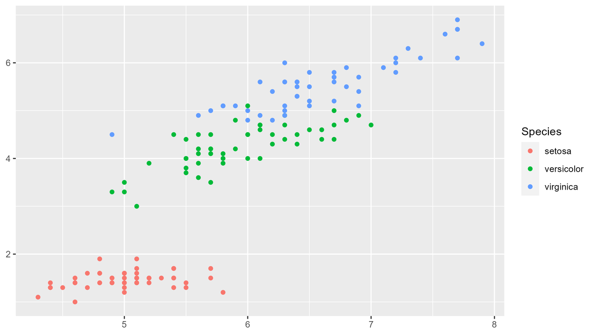
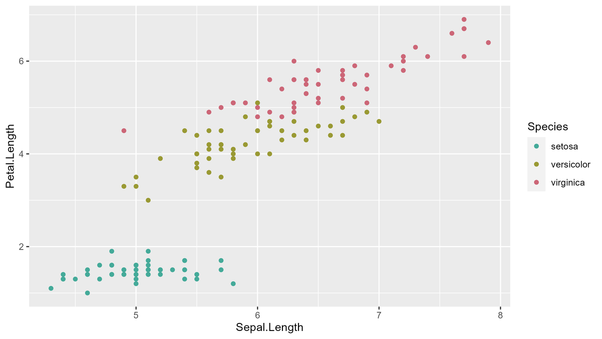
基本編

##Species毎に散布図を書く
iris %>%
  ggplot(aes(x=Sepal.Length, y=Petal.Length, color = Species))+
  geom_point()

##Petal.Widthで色付けして散布図を書く
iris %>%
  ggplot(aes(x=Sepal.Length, y=Petal.Length, color = Petal.Width))+
  geom_point()

条件合致のみプロット編

##Petal.Widthが0.4以上、1.8以下のものを抜き出して散布図を書く
iris %>%
  dplyr::filter(Petal.Width >= 0.40, Petal.Width <= 1.8) %>%
  ggplot(aes(x=Sepal.Length, y=Petal.Length, color = Species))+
  geom_point()

##virginicaのみを抜き出して散布図を書く
iris %>%
  dplyr::filter(Species == "virginica") %>%
  ggplot(aes(x=Sepal.Length, y=Petal.Length, color = Species))+
  geom_point()

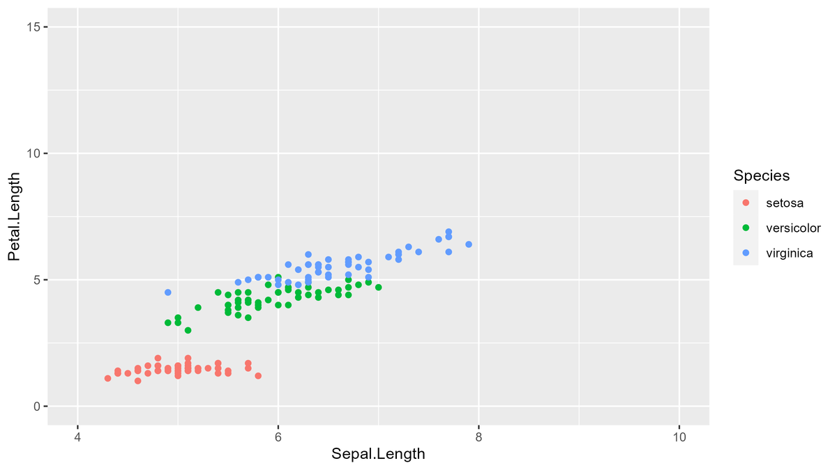
軸の調整編

##軸の範囲を変更する（枠外も考慮するため推奨）
iris %>%
  ggplot(aes(x=Sepal.Length, y=Petal.Length, color = Species))+
  geom_point()+
  coord_cartesian(xlim=c(4,10),ylim=c(0,15))

##軸の範囲を変更する（枠外を無視するため非推奨）
iris %>%
  ggplot(aes(x=Sepal.Length, y=Petal.Length, color = Species))+
  geom_point()+
  ylim(0,15)+
  xlim(4,10)

##軸の範囲と区切り線の単位を変更する
iris %>%
  ggplot(aes(x=Sepal.Length, y=Petal.Length, color = Species))+
  geom_point()+
  coord_cartesian(xlim=c(4,10),ylim=c(0,15))+
  scale_x_continuous(breaks = seq(4,10,by=0.5))+
  scale_y_continuous(breaks = seq(0,15,length=16))

軸ラベルやタイトル編

##軸のラベルを変更する
iris %>%
  ggplot(aes(x=Sepal.Length, y=Petal.Length, color = Species))+
  geom_point()+
  labs(x = "NEW X LABEL", y = "NEW Y LABEL", color = "NEW COLOR LABEL")

##軸のラベルを消す
iris %>%
  ggplot(aes(x=Sepal.Length, y=Petal.Length, color = Species))+
  geom_point()+
  theme(axis.title.x = element_blank(),axis.title.y = element_blank())

##グラフのタイトルを変更する
iris %>%
  ggplot(aes(x=Sepal.Length, y=Petal.Length, color = Species))+
  geom_point()+
  labs(title = "NEW TITLE 1")

##グラフのタイトルを変更して位置を調整する
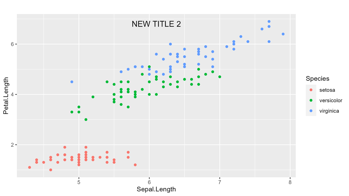
iris %>%
  ggplot(aes(x=Sepal.Length, y=Petal.Length, color = Species))+
  geom_point()+
  ggtitle("NEW TITLE 2")+
  theme(plot.title = element_text(hjust = 0.5, vjust = -10))

点の見た目の変更編

##点のサイズと形状を変更する
iris %>%
  ggplot(aes(x=Sepal.Length, y=Petal.Length, color = Species))+
  geom_point(shape = 4, size = 3)

色の調整編

##自分で指定した任意の色でプロットする①
iris %>%
  ggplot(aes(x=Sepal.Length, y=Petal.Length, color = Species))+
  geom_point()+
  scale_color_manual(values = c(setosa = "#FF4B00",
                                versicolor = "#005AFF",
                                virginica = "#03AF7A" ))

##自分で指定した任意の色でプロットする②
iris %>%
  ggplot(aes(x=Sepal.Length, y=Petal.Length, color = Species))+
  geom_point()+
  scale_color_manual(values = c("#44AA99","#999933","#CC6677"))


##colorの色分けを自分で決めたカラーパレットにする
pal <- c("#3B9AB2","#53A5B9","#6BB1C1","#8FBBA5","#BDC367",
         "#EBCC2A","#E6C019","#E3B408","#E49100","#EB5500","#F21A00")
iris %>%
  ggplot(aes(x=Sepal.Length, y=Petal.Length, color = Petal.Width))+
  geom_point() +
  scale_color_gradientn(colors = pal) 
                  
##色付けscale_color_gradientnの範囲を定める
pal <- c("#3B9AB2","#53A5B9","#6BB1C1","#8FBBA5","#BDC367",
         "#EBCC2A","#E6C019","#E3B408","#E49100","#EB5500","#F21A00")
iris %>%
  ggplot(aes(x=Sepal.Length, y=Petal.Length, color = Petal.Width))+
  geom_point() +
  scale_color_gradientn(colors = pal,limits=c(0.5,2.0))

並べてプロット編

##Species毎にgridで並べる（gridの横軸にSpecies）
iris %>%
  ggplot(aes(x=Sepal.Length, y=Petal.Length, color = Species))+
  geom_point()+
  facet_grid(. ~ Species, scales = "fixed")

##Species毎にgridで並べる（gridの縦軸にSpecies）
iris %>%
  ggplot(aes(x=Sepal.Length, y=Petal.Length, color = Species))+
  geom_point()+
  facet_grid(Species ~ ., scales = "free")

##Species毎に別々の図で並べる
iris %>%
  ggplot(aes(x=Sepal.Length, y=Petal.Length, color = Species))+
  geom_point()+
  facet_wrap(~Species, nrow=2, scales = "free_y")

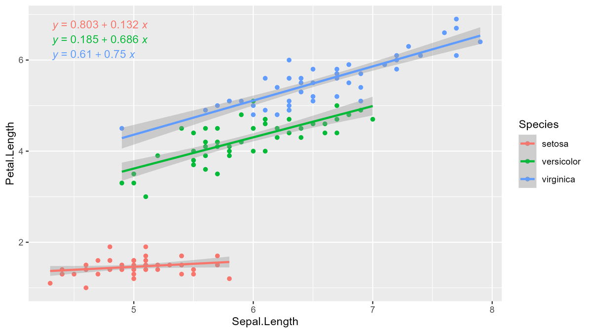
回帰直線編

##それっぽい回帰直線を引く
library(ggpmisc)
iris %>%
  ggplot(aes(x=Sepal.Length, y=Petal.Length, color = Species))+
  geom_point()+
  geom_smooth(method="lm",aes(color=Species),se=TRUE)+
  stat_poly_eq(formula = y ~ x,
                 aes(label = paste(stat(eq.label))),
                 parse = TRUE)

##相関係数を載せる
library(ggpmisc)
iris %>%
  ggplot(aes(x=Sepal.Length, y=Petal.Length, color = Species))+
  geom_point()+
  geom_smooth(method="lm",aes(color=Species),se=TRUE)+
  stat_poly_eq(aes(label = paste(stat(rr.label))),
               label.x = "right",label.y = "bottom",
               parse = TRUE)

##回帰直線の式と相関係数を両方載せる
library(ggpmisc)
iris %>%
  ggplot(aes(x=Sepal.Length, y=Petal.Length, color = Species))+
  geom_point()+
  geom_smooth(method="lm",aes(color=Species),se=TRUE)+
  stat_poly_eq(formula = y ~ x,
               aes(label = paste(stat(eq.label))),
               parse = TRUE)+
  stat_poly_eq(aes(label = paste(stat(rr.label))),
               label.x = "right",label.y = "bottom",
               parse = TRUE)

その他

##データの値を1000倍して散布図を書く
iris %>%
  mutate(Sepal.Length = Sepal.Length * 1000,
         Petal.Length = Petal.Length * 1000) %>%
  ggplot(aes(x=Sepal.Length, y=Petal.Length, color = Species))+
  geom_point()

実施例

基本編

##Species毎に散布図を書く
iris %>%
  ggplot(aes(x=Sepal.Length, y=Petal.Length, color = Species))+
  geom_point()

##Petal.Widthで色付けして散布図を書く
iris %>%
  ggplot(aes(x=Sepal.Length, y=Petal.Length, color = Petal.Width))+
  geom_point()

条件合致のみプロット編

##Petal.Widthが0.4以上、1.8以下のものを抜き出して散布図を書く
iris %>%
  dplyr::filter(Petal.Width >= 0.40, Petal.Width <= 1.8) %>%
  ggplot(aes(x=Sepal.Length, y=Petal.Length, color = Species))+
  geom_point()

##virginicaのみを抜き出して散布図を書く
iris %>%
  dplyr::filter(Species == "virginica") %>%
  ggplot(aes(x=Sepal.Length, y=Petal.Length, color = Species))+
  geom_point()

軸の調整編

##軸の範囲を変更する（枠外も考慮するため推奨）
iris %>%
  ggplot(aes(x=Sepal.Length, y=Petal.Length, color = Species))+
  geom_point()+
  coord_cartesian(xlim=c(4,10),ylim=c(0,15))

##軸の範囲を変更する（枠外を無視するため非推奨）
iris %>%
  ggplot(aes(x=Sepal.Length, y=Petal.Length, color = Species))+
  geom_point()+
  ylim(0,15)+
  xlim(4,10)

##軸の範囲と区切り線の単位を変更する
iris %>%
  ggplot(aes(x=Sepal.Length, y=Petal.Length, color = Species))+
  geom_point()+
  coord_cartesian(xlim=c(4,10),ylim=c(0,15))+
  scale_x_continuous(breaks = seq(4,10,by=0.5))+
  scale_y_continuous(breaks = seq(0,15,length=16))

軸ラベルやタイトル編

##軸のラベルを変更する
iris %>%
  ggplot(aes(x=Sepal.Length, y=Petal.Length, color = Species))+
  geom_point()+
  labs(x = "NEW X LABEL", y = "NEW Y LABEL", color = "NEW COLOR LABEL")

##軸のラベルを消す
iris %>%
  ggplot(aes(x=Sepal.Length, y=Petal.Length, color = Species))+
  geom_point()+
  theme(axis.title.x = element_blank(),axis.title.y = element_blank())

##グラフのタイトルを変更する
iris %>%
  ggplot(aes(x=Sepal.Length, y=Petal.Length, color = Species))+
  geom_point()+
  labs(title = "NEW TITLE 1")

##グラフのタイトルを変更して位置を調整する
iris %>%
  ggplot(aes(x=Sepal.Length, y=Petal.Length, color = Species))+
  geom_point()+
  ggtitle("NEW TITLE 2")+
  theme(plot.title = element_text(hjust = 0.5, vjust = -10))

点の見た目の変更編

##点のサイズと形状を変更する
iris %>%
  ggplot(aes(x=Sepal.Length, y=Petal.Length, color = Species))+
  geom_point(shape = 4, size = 3)

色の調整編

##自分で指定した任意の色でプロットする①
iris %>%
  ggplot(aes(x=Sepal.Length, y=Petal.Length, color = Species))+
  geom_point()+
  scale_color_manual(values = c(setosa = "#FF4B00",
                                versicolor = "#005AFF",
                                virginica = "#03AF7A" ))

##自分で指定した任意の色でプロットする②
iris %>%
  ggplot(aes(x=Sepal.Length, y=Petal.Length, color = Species))+
  geom_point()+
  scale_color_manual(values = c("#44AA99","#999933","#CC6677"))

##colorの色分けを自分で決めたカラーパレットにする
pal <- c("#3B9AB2","#53A5B9","#6BB1C1","#8FBBA5","#BDC367",
         "#EBCC2A","#E6C019","#E3B408","#E49100","#EB5500","#F21A00")
iris %>%
  ggplot(aes(x=Sepal.Length, y=Petal.Length, color = Petal.Width))+
  geom_point() +
  scale_color_gradientn(colors = pal)

##色付けscale_color_gradientnの範囲を定める
pal <- c("#3B9AB2","#53A5B9","#6BB1C1","#8FBBA5","#BDC367",
         "#EBCC2A","#E6C019","#E3B408","#E49100","#EB5500","#F21A00")
iris %>%
  ggplot(aes(x=Sepal.Length, y=Petal.Length, color = Petal.Width))+
  geom_point() +
  scale_color_gradientn(colors = pal,limits=c(0.5,2.0))

並べてプロット編

##Species毎にgridで並べる（gridの横軸にSpecies）
iris %>%
  ggplot(aes(x=Sepal.Length, y=Petal.Length, color = Species))+
  geom_point()+
  facet_grid(. ~ Species, scales = "fixed")

##Species毎にgridで並べる（gridの縦軸にSpecies）
iris %>%
  ggplot(aes(x=Sepal.Length, y=Petal.Length, color = Species))+
  geom_point()+
  facet_grid(Species ~ ., scales = "free")

##Species毎に別々の図で並べる
iris %>%
  ggplot(aes(x=Sepal.Length, y=Petal.Length, color = Species))+
  geom_point()+
  facet_wrap(~Species, nrow=2, scales = "free_y")

回帰直線編

##それっぽい回帰直線を引く
library(ggpmisc)
iris %>%
  ggplot(aes(x=Sepal.Length, y=Petal.Length, color = Species))+
  geom_point()+
  geom_smooth(method="lm",aes(color=Species),se=TRUE)+
  stat_poly_eq(formula = y ~ x,
                 aes(label = paste(stat(eq.label))),
                 parse = TRUE)

##相関係数を載せる
library(ggpmisc)
iris %>%
  ggplot(aes(x=Sepal.Length, y=Petal.Length, color = Species))+
  geom_point()+
  geom_smooth(method="lm",aes(color=Species),se=TRUE)+
  stat_poly_eq(aes(label = paste(stat(rr.label))),
               label.x = "right",label.y = "bottom",
               parse = TRUE)

##回帰直線の式と相関係数を両方載せる
library(ggpmisc)
iris %>%
  ggplot(aes(x=Sepal.Length, y=Petal.Length, color = Species))+
  geom_point()+
  geom_smooth(method="lm",aes(color=Species),se=TRUE)+
  stat_poly_eq(formula = y ~ x,
               aes(label = paste(stat(eq.label))),
               parse = TRUE)+
  stat_poly_eq(aes(label = paste(stat(rr.label))),
               label.x = "right",label.y = "bottom",
               parse = TRUE)

その他

##データの値を1000倍して散布図を書く
iris %>%
  mutate(Sepal.Length = Sepal.Length * 1000,
         Petal.Length = Petal.Length * 1000) %>%
  ggplot(aes(x=Sepal.Length, y=Petal.Length, color = Species))+
  geom_point()